Diamond Version 5 User Manual: Data sheet and powder pattern

Powder pattern simulation

In this article:
Powder diffraction data can be calculated and displayed in both table and diagram and update automatically when structure parameters change.
- Activating the powder pattern view
- Powder pattern settings
- Diffraction diagram settings.

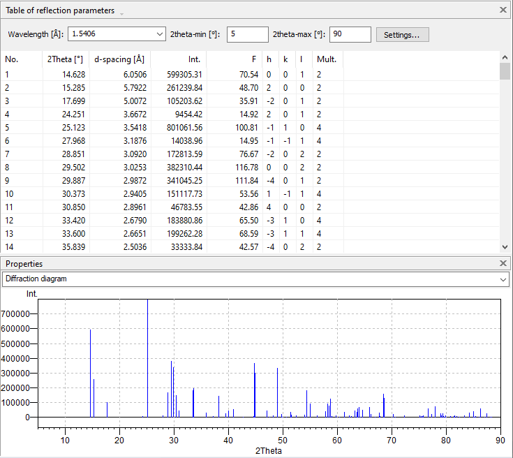
Previous article: Customizing a data sheet
Next article: Copying, Saving, and Printing Data from the Data Sheet or Powder Pattern

Activating the powder pattern view

Like the data sheet or the several object tables, and the table of distances and angles, the powder pattern is displayed in the secondary pane (data pane) of the structure window. The table of reflection parameters is placed in the upper part, i.e. where data sheet and the other tables are located, whereas the diffraction diagram is placed in the Properties pane below the table.

To open both table of reflection parameters and diffraction diagram, choose the Powder Pattern command from the View menu. If the secondary pane has not yet been opened, the mouse cursor will change to split mode, that means you can shift the border line between graphics and data pane to adjust the appropriate width for the table of reflection parameters and the diffraction diagram.

The powder pattern view can also be activated with the corresponding button in the main toolbar: 

Screenshot of sample PCD-VxOy.cif with "455496" focused: Reflection parameter table in the upper part of the data pane, the diffraction diagram in the lower part (in the properties pane)

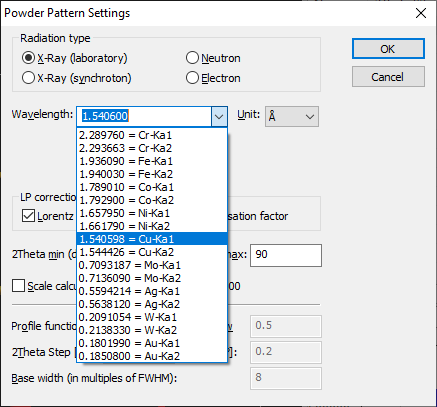
Powder Pattern Settings

A small dialog bar with the most common settings for a powder pattern is above the table of reflection parameters:

Wavelength
Here, you can enter the wavelength of the X-ray radiation that is used for the calculation of the powder diffraction pattern. Once you have entered or selected the wavelength of the radiation, press Return in order to update the reflection list and the diffraction pattern.

2theta-min and 2theta-max
You can define a lower and an upper 2theta limit for the calculation of the peaks/reflections (in Å). Especially the upper 2theta limit is generally useful for short wavelengths and/or large unit cells in order to reduce the calculation time. Once you have modified at least one of these values, use the Return key in order to update the reflection list and the diffraction pattern.

Sorting the reflection parameters

By default, the reflection parameters are sorted for increasing 2theta values. You can change the sort order in the table of reflection parameters for each column, simply by clicking on the corresponding column header.

Profile and other powder pattern settings

More settings are available through the Settings button, which opens the Powder Pattern Settings dialog where you can define the radiation type, the wavelength, the Lorentz-Polarization correction, and the 2theta limits. Here you also decide whether you would like to display the diffraction pattern either as a "stick pattern" (peaks only) or as profile, along with the profile parameters (e.g. FWHM).

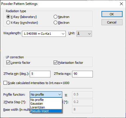
In the upper part of the dialog, you define radiation type, wavelength and unit, correction, and an optional scaling of intensities:

Radiation type
Defines the type of radiation which shall be used in the diffraction pattern calculation:

• X-Ray (laboratory): This is the default setting. Most powder diffraction patterns are measured on conventional laboratory X-ray diffractometers.
• X-Ray (synchrotron): Synchrotron X-ray diffraction data; in this case, the polarization correction (see LP correction below) is disabled automatically.
• Neutron: In certain cases (e.g. if the positions of very light atoms like H have to determined in the presence of very heavy atoms) it is convenient to use neutron radiation. The polarization correction is disabled automatically.
• Electron: The calculation of electron diffraction data is also possible. However, dynamical diffraction is ignored.

Wavelength
Defines the wavelength of the radiation in Angstroem (Å). The default is X-ray Cu K α 1 radiation (1.540598 Å).

LP correction
In this field, you indicate which correction should be applied to the calculated powder patterns. For instance, for conventional laboratory X-ray diffractometers you would use both corrections (Lorentz- and polarisation correction) and hence check both fields. With X-ray synchrotron as well as neutron diffraction data, you would generally leave the Polarisation correction unchecked.

2theta min
Defines the lower boundary value of the 2theta range used to calculate the diffraction pattern. This value may be used together with the 2Theta max value to select a "window" of relevant peaks.

2theta max
Defines the upper boundary value of the 2theta range of the calculated diffraction pattern. This value may be used together with the 2Theta min value to select a "window" of relevant peaks. This is also generally useful for short wavelengths and/or large unit cells in order to reduce the calculation time.

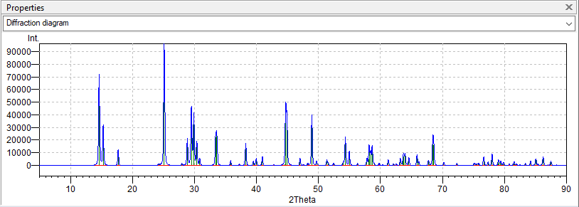
Scale calculated intensities to Int.max = 1000
If this box is checked, the intensities of the diffraction pattern calculated for the current structural model will be scaled to a maximum value of 1000.

Using a profile function or not

The powder diffraction pattern can either be displayed as "stick pattern" (peaks) or as "profile pattern". By default, the option Profile function is set to "No profile", resulting in the stick pattern representation. However, you can also display the diffraction pattern as a profile by selecting a profile function (and adjusting the corresponding parameters):

w
This value defines the Pseudo-Voigt weighting factor and is used to increase or decrease the Lorentzian (L(ik)) or Gaussian (G(ik)) part:

y(ik) = w * L(ik) + (1 - w) * G(ik)

This factor must be in the range from 0 through 1, where w = 0 means Gaussian only and w = 1 means Lorentzian only.

2Theta Step
This defines the width between two data points, given in degrees 2theta, that is used to calculate the y-data points (y(ik)) for the profiles.

FWHM
This means "full width at half maximum" and is the full width, in degrees 2theta, used to define the width of each profile in the diffraction diagram.

Base width
This factor, given as a multiple of the FWHM parameter, defines where the calculation of the y(ik) values of the left or right half of a single profile stops. (Gaussian and Lorentzian function do not reach 0 but go asymptotically against 0.)

The same diffraction diagram as above but here with Pseudo-Voigt profile function activated.

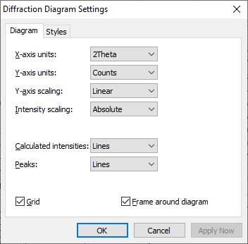
Diffraction Diagram Settings

The context menu of the diffraction diagram in the properties pane (available e.g. by clicking on the right mouse button inside the diagram), offers several settings:

Zooming
If the diffraction pattern is in the (default) "zooming" mode (which can be selected from the Mode context menu), you can select a certain area of the pattern with your mouse (simply move to the left (lower) boundary you want to select, press the mouse button, and move to the right (upper) boundary of the area of which you want to see further details). Once you release the mouse button, only this area will be shown instead of the whole diffraction pattern. If you want to go back to the full pattern, please select the Zoom out command from the context menu. Alternatively, you can also go back to the previous zoom by selecting the corresponding command from the context menu.

Tracking
In this mode (which can be activated in the Mode context menu), you can zoom and move through the diffraction pattern at the same time, as long as you keep the mouse button pressed. A mouse movement up or down enlarges or diminishes the scaling factor, while a mouse movement to the left or right will scroll through the pattern. Thus, you can easily move to an interesting part of the diffraction pattern and zoom into its details at the same time with a single mouse operation.

Diagram Settings...
This command opens the Diffraction Diagram Settings dialog where you can define the units of the x- and y-axis of the diffraction pattern, the scaling, the colors used in the diagram etc.

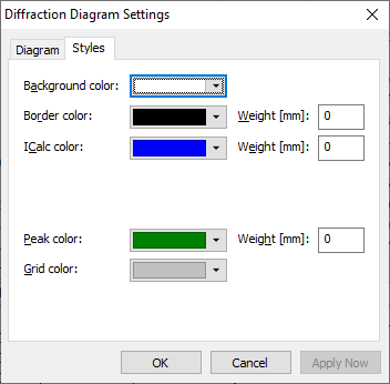
Defining axes' units and scaling

The Diffraction Diagram Settings dialog has two pages. You define the units and the scalings (or stretchings) for x- and y-axis on the first page:

The X-axis units can be: theta, 2theta, and 4theta, all in degrees. Besides this you can use sin²theta as well as d-spacings in Angstroem. The default is 2theta.

Y-axis units: This defines if the intensity values on the y-axis are to be scaled relative to 1000 or not. By default, the y-axis uses unscaled intensities, calculated from F-values, in the range of about 1e6 to 1e12, depending on the size of the unit cell. This is called "Counts".

Y-axis scaling defines if the intensities on the y-axis are to be displayed linear, i.e. without scaling, or scaled. Scaling enlarges small intensities relative to the strong ones. There are two options to scale: Using the square root values of the intensities or logarithmic values.

Intensity scaling

There are three options, if and how to scale the highest peak within a given "peak window" (part of the total 2theta or d-spacing range):

Absolute: The "strongest peak" (highest intensity value) reaches the top of the diagram, the residual peaks are stretched relative to that peak.

Relative: If you display only a portion of the diffraction diagram (a "2theta window"), the intensities will be maximized so that the strongest peak in the current 2theta window reaches the top of the diagram.

No scaling: Switching to this option "freezes" the current scaling. This means, after stretching peaks within a 2theta window using the Relative option and then switching to No scaling, the scaling does not change even if you move to stronger peaks outside the previous 2theta window.

Showing peaks or not

Calculated intensities defines if to display peaks as lines or to hide calculated peaks.

The Peaks option refers to display of peaks when displaying profile data. You can either display the peaks as lines, as bars or do not display them at all ("Hide"). If "Bars" is selected, the width of the bars will be equivalent to the full width at half maximum (FWHM).

Grid and frame

If the Grid checkbox is activated, dotted lines are used for 10-degree 2theta units as well as for the superior y-values.

If the Frame around diagram checkbox is activated, a frame is drawn around the diffraction diagram. Otherwise, only the x- and y-axis are drawn.

Defining colors and line styles of the diffraction diagram

These are defined on the Styles page of the Diffraction Diagram Settings dialog:

Background color defines the color used for the background of the diffraction diagram.

Border color defines the color used for the x- and y-axis as well as for the border (frame) of the diagram. Besides this, you can adjust the width of the borders ("Weight", given in mm).

ICalc color defines the color used for the calculated peaks or profile. Besides this, you can adjust the width of the peaks or profile line ("Weight", given in mm).

Peak color: This color is used for peak lines or bars used in profile display. Besides this, you can adjust the width of the peak lines ("Weight", given in mm).

Grid color: This color is used to draw the horizontal and vertical lines of the grid.

Previous article: Customizing a data sheet
Next article: Copying, Saving, and Printing Data from the Data Sheet or Powder Pattern

[1] ICSD: 23119: Jackson P F, Johnson B F G, Lewis J, Nicholls J N, McPartlin M, Nelson W J H; "Synthesis of the Carbido Anion (Os₅ C (C O)₁₅ I)and the X-Ray Crystal Structures of Os₅ C (C O)₁₅ and Ph₃ P)₂ N) (Os₅ C (C O)₁₅ I)". JCCCA, 1980, 564-566 (1980).